这篇文章主要介绍“Python+OpenCV怎么解决彩色图亮度不均衡问题”,在日常操作中,相信很多人在Python+OpenCV怎么解决彩色图亮度不均衡问题问题上存在疑惑,小编查阅了各式资料,整理出简单好用的操作方法,希望对大家解答”Python+OpenCV怎么解决彩色图亮度不均衡问题”的疑惑有所帮助!接下来,请跟着小编一起来学习吧!
也就是把图像重新缩放到指定的范围内
# 对比度拉伸
p1, p2 = np.percentile(img, (0, 70))  # numpy计算多维数组的任意百分比分位数
rescale_img = np.uint8((np.clip(img, p1, p2) - p1) / (p2 - p1) * 255)其中,numpy的percentile函数可以计算多维数组的任意百分比分位数,因为我的图片中整体偏暗,我就把原图灰度值的0% ~ 70%缩放到0 ~255
使用以下公式进行映射:
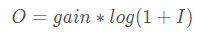
# 对数变换
log_img = np.zeros_like(img)
scale, gain = 255, 1.5
for i in range(3):
log_img[:, :, i] = np.log(img[:, :, i] / scale + 1) * scale * gain使用以下公式进行映射:
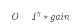
# gamma变换
gamma, gain, scale = 0.7, 1, 255
gamma_img = np.zeros_like(img)
for i in range(3):
gamma_img[:, :, i] = ((img[:, :, i] / scale) ** gamma) * scale * gain使用直方图均衡后的图像具有大致线性的累积分布函数,其优点是不需要参数。
其原理为,考虑这样一个图像,它的像素值被限制在某个特定的值范围内,即灰度范围不均匀。所以我们需要将其直方图缩放遍布整个灰度范围(如下图所示,来自维基百科),这就是直方图均衡化所做的(简单来说)。这通常会提高图像的对比度。
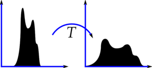
这里使用OpenCV来演示。
# 直方图均衡化
equa_img = np.zeros_like(img)
for i in range(3):
equa_img[:, :, i] = cv.equalizeHist(img[:, :, i])这是一种自适应直方图均衡化方法
OpenCV提供了该方法。
# 对比度自适应直方图均衡化
clahe_img = np.zeros_like(img)
clahe = cv.createCLAHE(clipLimit=2.0, tileGridSize=(8, 8))
for i in range(3):
clahe_img[:, :, i] = clahe.apply(img[:, :, i])使用Matplotlib显示上述几种方法的结果:
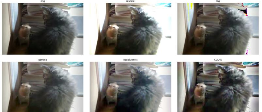
可以看到,前四种方法效果都差不多,都有一个问题亮的地方过于亮,这是因为他们考虑的是全局对比度,而且因为我们使用的彩色图像原因,使用log变换的结果图中有部分区域色彩失真。最后一种CLAHE方法考虑的是局部对比度,所以效果会好一点。
因为图像是彩色的,这里我只绘制了R通道的直方图(红色线)及其累积分布函数(黑色线)
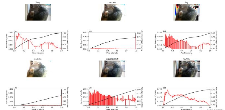
可以看到均衡后的图像具有大致线性的累积分布函数。
总之,经过以上的探索,我最终决定使用CLAHE均衡后的结果,感觉是比之前的好了点
import cv2.cv2 as cv
import matplotlib.pyplot as plt
import numpy as np


def plot_img_and_hist(image, axes, bins=256):
    """Plot an image along with its histogram and cumulative histogram.

    """
    ax_img, ax_hist = axes
    ax_cdf = ax_hist.twinx()

    # Display image
    ax_img.imshow(image, cmap=plt.cm.gray)
    ax_img.set_axis_off()

    # Display histogram
    colors = ['red', 'green', 'blue']
    for i in range(1):
        ax_hist.hist(image[:, :, i].ravel(), bins=bins, histtype='step', color=colors[i])

    ax_hist.ticklabel_format(axis='y', style='scientific', scilimits=(0, 0))

    ax_hist.set_xlabel('Pixel intensity')
    ax_hist.set_xlim(0, 255)    # 这里范围为0~255 如果使用img_as_float,则这里为0~1
    ax_hist.set_yticks([])

    # Display cumulative distribution
    for i in range(1):
        hist, bins = np.histogram(image[:, :, i].flatten(), 256, [0, 256])
        cdf = hist.cumsum()
        cdf = cdf * float(hist.max()) / cdf.max()
        ax_cdf.plot(bins[1:], cdf, 'k')
    ax_cdf.set_yticks([])

    return ax_img, ax_hist, ax_cdf


def plot_all(images, titles, cols):
    """
    输入titles、images、以及每一行多少列,自动计算行数、并绘制图像和其直方图
    :param images:
    :param titles:
    :param cols: 每一行多少列
    :return:
    """
    fig = plt.figure(figsize=(12, 8))
    img_num = len(images)  # 图片的个数
    rows = int(np.ceil(img_num / cols) * 2)  # 上图下直方图 所以一共显示img_num*2个子图
    axes = np.zeros((rows, cols), dtype=object)
    axes = axes.ravel()
    axes[0] = fig.add_subplot(rows, cols, 1)  # 先定义第一个img 单独拿出来定义它是为了下面的sharex
    # 开始创建所有的子窗口
    for i in range(1, img_num):  #
        axes[i + i // cols * cols] = fig.add_subplot(rows, cols, i + i // cols * cols + 1, sharex=axes[0],
                                                     sharey=axes[0])
    for i in range(0, img_num):
        axes[i + i // cols * cols + cols] = fig.add_subplot(rows, cols, i + i // cols * cols + cols + 1)

    for i in range(0, img_num):  # 这里从1开始,因为第一个在上面已经绘制过了
        ax_img, ax_hist, ax_cdf = plot_img_and_hist(images[i],
                                                    (axes[i + i // cols * cols], axes[i + i // cols * cols + cols]))
        ax_img.set_title(titles[i])
        y_min, y_max = ax_hist.get_ylim()
        ax_hist.set_ylabel('Number of pixels')
        ax_hist.set_yticks(np.linspace(0, y_max, 5))

        ax_cdf.set_ylabel('Fraction of total intensity')
        ax_cdf.set_yticks(np.linspace(0, 1, 5))

    # prevent overlap of y-axis labels
    fig.tight_layout()
    plt.show()
    plt.close(fig)


if __name__ == '__main__':
    img = cv.imread('catandmouse.png', cv.IMREAD_UNCHANGED)[:, :, :3]
    img = cv.cvtColor(img, cv.COLOR_BGR2RGB)

    gray = cv.cvtColor(img, cv.COLOR_BGR2GRAY)
    # 对比度拉伸
    p1, p2 = np.percentile(img, (0, 70))  # numpy计算多维数组的任意百分比分位数
    rescale_img = np.uint8((np.clip(img, p1, p2) - p1) / (p2 - p1) * 255)

    # 对数变换
    log_img = np.zeros_like(img)
    scale, gain = 255, 1.5
    for i in range(3):
        log_img[:, :, i] = np.log(img[:, :, i] / scale + 1) * scale * gain

    # gamma变换
    gamma, gain, scale = 0.7, 1, 255
    gamma_img = np.zeros_like(img)
    for i in range(3):
        gamma_img[:, :, i] = ((img[:, :, i] / scale) ** gamma) * scale * gain

    # 彩色图直方图均衡化
    # 直方图均衡化
    equa_img = np.zeros_like(img)
    for i in range(3):
        equa_img[:, :, i] = cv.equalizeHist(img[:, :, i])
    # 对比度自适应直方图均衡化
    clahe_img = np.zeros_like(img)
    clahe = cv.createCLAHE(clipLimit=2.0, tileGridSize=(8, 8))
    for i in range(3):
        clahe_img[:, :, i] = clahe.apply(img[:, :, i])

    titles = ['img', 'rescale', 'log', 'gamma', 'equalizeHist', 'CLAHE']
    images = [img, rescale_img, log_img, gamma_img, equa_img, clahe_img]
plot_all(images, titles, 3)from skimage import exposure, util, io, color, filters, morphology
import matplotlib.pyplot as plt
import numpy as np
def plot_img_and_hist(image, axes, bins=256):
"""Plot an image along with its histogram and cumulative histogram.
"""
image = util.img_as_float(image)
ax_img, ax_hist = axes
ax_cdf = ax_hist.twinx()
# Display image
ax_img.imshow(image, cmap=plt.cm.gray)
ax_img.set_axis_off()
# Display histogram
colors = ['red', 'green', 'blue']
for i in range(1):
ax_hist.hist(image[:, :, i].ravel(), bins=bins, histtype='step', color=colors[i])
ax_hist.ticklabel_format(axis='y', style='scientific', scilimits=(0, 0))
ax_hist.set_xlabel('Pixel intensity')
ax_hist.set_xlim(0, 1)
ax_hist.set_yticks([])
# Display cumulative distribution
for i in range(1):
img_cdf, bins = exposure.cumulative_distribution(image[:, :, i], bins)
ax_cdf.plot(bins, img_cdf, 'k')
ax_cdf.set_yticks([])
return ax_img, ax_hist, ax_cdf
def plot_all(images, titles, cols):
"""
输入titles、images、以及每一行多少列,自动计算行数、并绘制图像和其直方图
:param images:
:param titles:
:param cols: 每一行多少列
:return:
"""
fig = plt.figure(figsize=(12, 8))
img_num = len(images) # 图片的个数
rows = int(np.ceil(img_num / cols) * 2) # 上图下直方图 所以一共显示img_num*2个子图
axes = np.zeros((rows, cols), dtype=object)
axes = axes.ravel()
axes[0] = fig.add_subplot(rows, cols, 1) # 先定义第一个img 单独拿出来定义它是为了下面的sharex
# 开始创建所有的子窗口
for i in range(1, img_num): #
axes[i + i // cols * cols] = fig.add_subplot(rows, cols, i + i // cols * cols + 1, sharex=axes[0],
sharey=axes[0])
for i in range(0, img_num):
axes[i + i // cols * cols + cols] = fig.add_subplot(rows, cols, i + i // cols * cols + cols + 1)
for i in range(0, img_num): # 这里从1开始,因为第一个在上面已经绘制过了
ax_img, ax_hist, ax_cdf = plot_img_and_hist(images[i],
(axes[i + i // cols * cols], axes[i + i // cols * cols + cols]))
ax_img.set_title(titles[i])
y_min, y_max = ax_hist.get_ylim()
ax_hist.set_ylabel('Number of pixels')
ax_hist.set_yticks(np.linspace(0, y_max, 5))
ax_cdf.set_ylabel('Fraction of total intensity')
ax_cdf.set_yticks(np.linspace(0, 1, 5))
# prevent overlap of y-axis labels
fig.tight_layout()
plt.show()
plt.close(fig)
if __name__ == '__main__':
img = io.imread('catandmouse.png')[:, :, :3]
gray = color.rgb2gray(img)
# 对比度拉伸
p1, p2 = np.percentile(img, (0, 70)) # numpy计算多维数组的任意百分比分位数
rescale_img = exposure.rescale_intensity(img, in_range=(p1, p2))
# 对数变换
# img = util.img_as_float(img)
log_img = np.zeros_like(img)
for i in range(3):
log_img[:, :, i] = exposure.adjust_log(img[:, :, i], 1.2, False)
# gamma变换
gamma_img = np.zeros_like(img)
for i in range(3):
gamma_img[:, :, i] = exposure.adjust_gamma(img[:, :, i], 0.7, 2)
# 彩色图直方图均衡化
equa_img = np.zeros_like(img, dtype=np.float64) # 注意直方图均衡化输出值为float类型的
for i in range(3):
equa_img[:, :, i] = exposure.equalize_hist(img[:, :, i])
# 对比度自适应直方图均衡化
clahe_img = np.zeros_like(img, dtype=np.float64)
for i in range(3):
clahe_img[:, :, i] = exposure.equalize_adapthist(img[:, :, i])
# 局部直方图均衡化 效果不好就不放了
selem = morphology.rectangle(50, 50)
loc_img = np.zeros_like(img)
for i in range(3):
loc_img[:, :, i] = filters.rank.equalize(util.img_as_ubyte(img[:, :, i]), footprint=selem)
# Display results
titles = ['img', 'rescale', 'log', 'gamma', 'equalizeHist', 'CLAHE']
images = [img, rescale_img, log_img, gamma_img, equa_img, clahe_img]
plot_all(images, titles, 3)到此,关于“Python+OpenCV怎么解决彩色图亮度不均衡问题”的学习就结束了,希望能够解决大家的疑惑。理论与实践的搭配能更好的帮助大家学习,快去试试吧!若想继续学习更多相关知识,请继续关注亿速云网站,小编会继续努力为大家带来更多实用的文章!
亿速云「云服务器」,即开即用、新一代英特尔至强铂金CPU、三副本存储NVMe SSD云盘,价格低至29元/月。点击查看>>
免责声明:本站发布的内容(图片、视频和文字)以原创、转载和分享为主,文章观点不代表本网站立场,如果涉及侵权请联系站长邮箱:is@yisu.com进行举报,并提供相关证据,一经查实,将立刻删除涉嫌侵权内容。


 计算
计算 安全
安全 数据库
数据库 网络和加速
网络和加速 企业服务
企业服务


