python中怎么模拟感知机算法

import numpy as np
import pandas as pd
# 导入数据集load_iris。
# 其中前四列为花萼长度，花萼宽度，花瓣长度，花瓣宽度等4个用于识别鸢尾花的属性，
from sklearn.datasets import load_iris
import matplotlib.pyplot as plot

# load data
iris = load_iris()

# 构造函数DataFrame(data,index,columns)，data为数据，index为行索引，columns为列索引
# 构造数据结构
df = pd.DataFrame(data=iris.data, columns=iris.feature_names)

# 在df中加入了新的一列：列名label的数据是target，即类型
# 第5列为鸢尾花的类别（包括Setosa，Versicolour，Virginica三类）。
# 也即通过判定花萼长度，花萼宽度，花瓣长度，花瓣宽度的尺寸大小来识别鸢尾花的类别。
df['label'] = iris.target
df.columns = ['sepal length', 'sepal width', 'petal length', 'petal width', 'label']

# 打印出label列值对应的数量。以及列名称、类型
# print(df.label.value_counts())

# 创建数组，
# 第一个参数:100表示取0-99行，即前100行；但100：表示100以后的所有数据。
# 第二个参数，0,1表示第一列和第二列，-1表示最后一列
data = np.array(df.iloc[:100, [0, 1, -1]])

# 数组切割，X切除了最后一列；y仅切最后一列
X, y = data[:, :-1], data[:, -1]

# 数据整理，将y中非1的改为-1
y = np.array([1 if i == 1 else -1 for i in y])

# 数据线性可分，二分类数据
# 此处为一元一次线性方程
class Model:
    def __init__(self):
        # w初始为自变量个数相同的（1,1）阵
        self.w = np.ones(len(data[0]) - 1, dtype=np.float32)
        self.b = 0
        # 学习率设置为0.1
        self.l_rate = 0.1

    def sign(self, x, w, b):
        # dot函数为点乘，区别于*乘。
        # dot对矩阵运算的时候为矩阵乘法，一行乘一列。
        # *乘对矩阵运算的时候，是对应元素相乘
        y = np.dot(x, w) + b
        return y

    # 随机梯度下降法
    def fit(self, X_train, y_train):
        is_wrong = False
        while not is_wrong:
            # 记录当前的分类错误的点数，当分类错误的点数归零的时候，即分类结束
            wrong_count = 0
            # d从0-49遍历
            for d in range(len(X_train)):
                # 这里的X为一行两列数组
                X = X_train[d]
                y = y_train[d]
                if y * self.sign(X, self.w, self.b) <= 0:
                    self.w = self.w + self.l_rate * np.dot(y, X)
                    self.b = self.b + self.l_rate * y
                    wrong_count += 1
            if wrong_count == 0:
                is_wrong = True
        return 'Perceptron Model!'

    def score(self):
        pass

perceptron = Model()
# 对perception进行梯度下降
perceptron.fit(X, y)

print(perceptron.w)
x_points = np.linspace(4, 7, 10)
# 最后拟合的函数瑞如下：
# w1*x1 + w2*x2 + b = 0
# 其中x1就是下边的x_points，x2就是y_
y_ = -(perceptron.w[0] * x_points + perceptron.b) / perceptron.w[1]
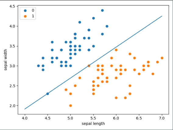
plot.plot(x_points, y_)

# scatter两个属性分别对应于x,y。
# 先画出了前50个点的花萼长度宽度，这时的花类型是0；
# 接着画50-100，这时花类型1
plot.scatter(df[:50]['sepal length'], df[:50]['sepal width'], label='0')
plot.scatter(df[50:100]['sepal length'], df[50:100]['sepal width'], label='1')
# 横坐标名称
plot.xlabel('sepal length')
# 纵坐标名称
plot.ylabel('sepal width')
plot.legend()
plot.show()

import sklearn
import pandas as pd
import numpy as np
import matplotlib.pyplot as plt
from sklearn.datasets import load_iris
from sklearn.linear_model import Perceptron

iris = load_iris()
df = pd.DataFrame(iris.data, columns=iris.feature_names)
df['label'] = iris.target
# df.columns = [
#     'sepal length', 'sepal width', 'petal length', 'petal width', 'label'
# ]
data = np.array(df.iloc[:100, [0, 1, -1]])
X, y = data[:, :-1], data[:, -1]
y = np.array([1 if i == 1 else -1 for i in y])

clf = Perceptron(fit_intercept=True,  # true表示估计截距
                 max_iter=1000,  # 训练数据的最大次数
                 shuffle=True,  # 每次训练之后是否重新训练
                 tol=None)  # 如果不设置none那么迭代将在误差小于1e-3结束
clf.fit(X, y)

# 输出粘合之后的w
print(clf.coef_)
# 输出拟合之后的截距b
print(clf.intercept_)

# 画布大小
plt.figure(figsize=(10, 10))

# 中文标题
# plt.rcParams['font.sans-serif'] = ['SimHei']
# plt.rcParams['axes.unicode_minus'] = False
# plt.title('鸢尾花线性数据示例')

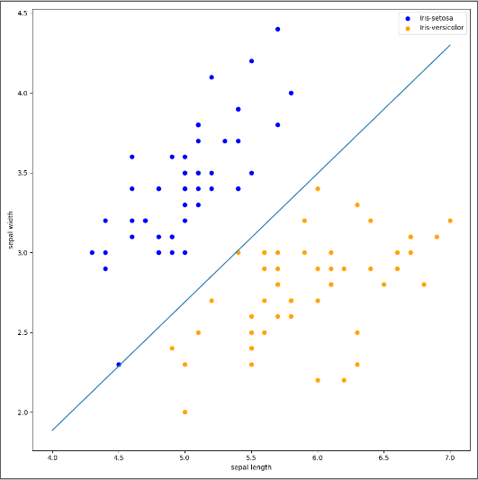
plt.scatter(data[:50, 0], data[:50, 1], c='b', label='Iris-setosa',)
plt.scatter(data[50:100, 0], data[50:100, 1], c='orange', label='Iris-versicolor')

# 画感知机的线
x_ponits = np.arange(4, 8)
y_ = -(clf.coef_[0][0]*x_ponits + clf.intercept_)/clf.coef_[0][1]
plt.plot(x_ponits, y_)

# 其他部分
plt.legend()  # 显示图例
plt.grid(False)  # 不显示网格
plt.xlabel('sepal length')
plt.ylabel('sepal width')
plt.legend()
plt.show()